

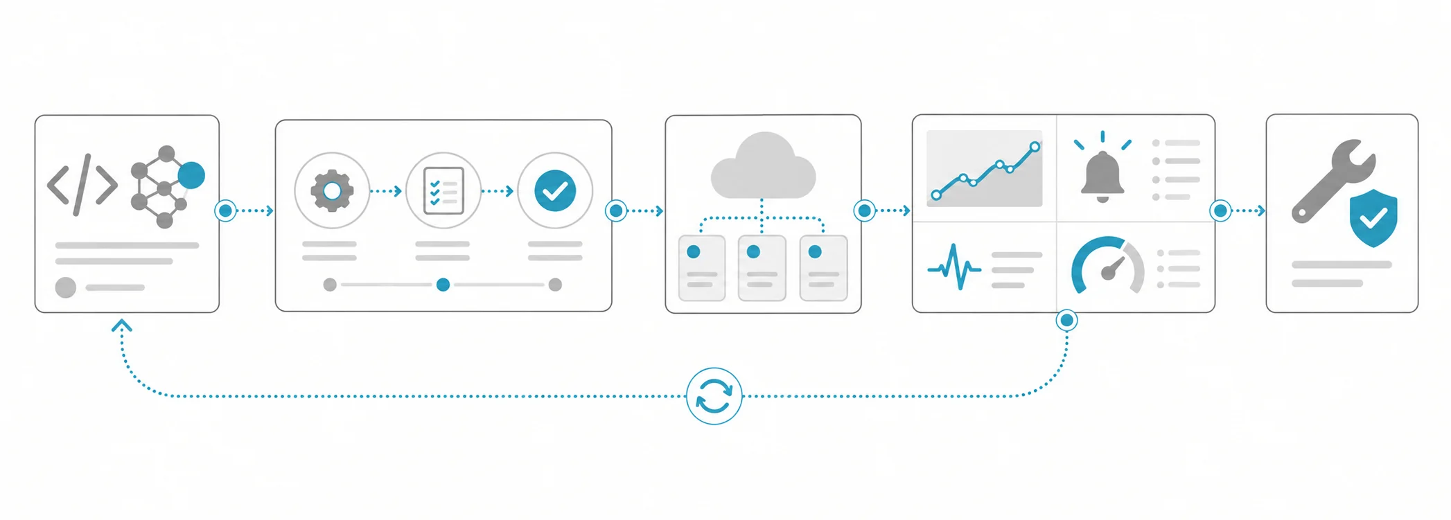
What is anomaly detection, and why use it in production?
Anomaly detection identifies examples that differ from an expected pattern. In visual quality control, a model built using only accepted part images learns normal appearance and assigns a difference score to a new image. It does not need to know the name or cause of every possible defect. When defects are rare, change shape or have no reliable labels yet, this approach can help establish a review channel.
A high anomaly score does not prove a defect. Lighting, camera angle, surface finish, product revision and harmless colour variation can also differ from the training images. The operational question is whether the inspection station can distinguish actionable defects from that variation. The model identifies differences from normal; the quality policy determines which differences are unacceptable. Do not assume these are the same decision.
The PatchCore paper describes an approach that builds a memory bank of regional features from normal images. The PaDiM paper models normal distributions of regional features extracted by a pretrained network. Both are research examples of anomaly detection and localisation. Which method works at your camera must be established on held-out production data. A published benchmark result cannot be transferred directly to a plant-specific acceptance claim.
How to design an evaluation for normal-only training
Training without defect labels does not mean evaluating without evidence. Normal examples measure false alerts. Measuring missed defects requires examples confirmed as defective by a specialist. You can keep those examples out of training and use them in a separate test. If you have no defect examples, limit the pilot's claim to review workload and robustness to normal variation rather than reporting an unsupported defect detection rate.
| Data group | Use | Protection rule |
|---|---|---|
| Normal training parts | Learn normal appearance | Confirmed acceptable examples |
| Normal validation parts | Select initial alert threshold | Different physical parts from training |
| Held-out normal test | Measure false alerts | Later batches and shifts |
| Confirmed defect test | Measure missed defects | Do not tune the threshold here |
| Live normal sample | Track drift under new conditions | Do not add automatically to retraining |
Do not distribute consecutive frames of the same part across these groups. Record how product variants and camera arrangements are represented. You may test a camera that was never present in training, but report that as performance under a new arrangement rather than blending it into results for established cameras. This makes the scope of each conclusion visible to the process owner.
Build the normal image set step by step
Collect accepted parts across shifts, machines, suppliers and product variants. Normal appearance is not just the flawless catalogue image: it includes surface and colour variation accepted by production. Confirm acceptance through quality records or specialist review. Remove questionable examples through a documented decision, rather than treating a high model score as sufficient reason to clean the dataset.
Keep the part ID, batch, camera, capture time, product revision, lighting settings and review decision with every image. These fields let you investigate where hidden defects entered the collection or under which conditions false alerts increased. Mark blurred, incomplete or incorrectly matched images separately. Build an image-quality check as a separate step rather than expecting the anomaly model to accept such images as normal.
Define the visible part region and the alignment rule. Crop out changing backgrounds or tray edges if they carry no information needed for the decision. Do not crop away a part edge where a defect could occur. Stabilising the camera and illumination helps interpret score distributions, but avoid excessive image correction that removes genuine product variation or hides a defect.
The MVTec AD 2 dataset provides normal training and validation images alongside normal and anomalous test images captured under differing lighting conditions. That arrangement is a useful reference for why a test that merely repeats training conditions is insufficient. Include shift, reflection and operating-condition differences in your own test. Results on the public dataset do not constitute an acceptance certificate for your product or station.
Set the alert threshold and the review path
Choose an initial threshold using the score distribution of normal validation images. For example, you can try a threshold corresponding to an agreed false-alert level on that group. This does not guarantee detection of unknown defects. Freeze the threshold and then evaluate it on independent normal and confirmed-defect tests. If you use defect examples to tune the threshold, allocate a separate validation group for them.
Distinguish the image score from the regional anomaly map. A map may help the operator locate a suspicious region, but do not assume it provides a validated measurement of physical area or a rejection boundary. Show the original image, highlighted region and relevant acceptance rule to the operator. Decision options can include accept, reject and uncertain. Record the reason: a click on an approval button alone is not enough to produce reliable evaluation data.
Record the model version, score calculation, threshold and approval date. Score scales may differ between model versions, so do not transfer an old threshold automatically to a replacement model. If missing a critical defect is expensive, run the system alongside the established inspection until sufficient evidence exists. Automatic rejection requires validated part identity and line timing as well as model performance, because the correct image decision must reach the correct physical part.
Hypothetical example: metal housing inspection
The following numbers are hypothetical and illustrate the calculation. Suppose metal housings are inspected with one overhead camera. There are 2,000 normal training images and 500 normal validation images from different parts. Keep 1,000 normal images from later batches and 40 confirmed scratch or dent images in a separate test. None of the defective images enters model training.
At the frozen threshold, suppose 20 of the 1,000 acceptable parts produce alerts, and 36 of the 40 defective parts produce alerts. The normal-test false-alert rate is 2%. Detection on the available defect test is 90%, with four missed defects. These percentages describe the limited sample of represented defect types. They do not establish that the same performance covers new defect shapes or other operating conditions.
If a shift processes 10,000 normal parts and the same false-alert rate persists, approximately 200 unnecessary reviews result. At 20 seconds per review, this requires about 67 minutes; reviews of real defects add to that workload. If night-shift reflections account for most alerts, investigate illumination first. Raising the threshold may reduce workload but can also increase missed defects, so evaluate the new selection using separate validation and test data.
A test plan and live monitoring
Expose results at the threshold you can actually operate, rather than relying only on a curve score. State that the false-alert denominator is the number of normal parts and the detection denominator is the number of confirmed defective parts. When defects are scarce, one example can change the percentage substantially. Keep the counts themselves in the report so that decision-makers can see the amount of evidence available.
- Independence: Audit training, validation and test separation using part and batch IDs. Check repeated captures as well as exact duplicate files, because distinct images may still show the same physical object.
- Difficult conditions: Measure each camera, shift, product variant and tiny-defect slice separately. Include the sample size and distinguish known arrangements from conditions that were absent from training.
- Workload: Calculate false alerts per thousand normal parts and review time per shift. Compare the queue with the people available to process it under the expected line throughput.
- Misses: Show missed examples by defect type. Do not write a success claim for a type with no confirmed examples in the test, even if its expected appearance seems unusual.
- Safe operation: Test the review path for missing images, late results and parts that cannot be found. Check that uncertain outcomes are recorded and do not silently become pass decisions.
When a camera, product or supplier changes, sample accepted images and inspect changes in alert rate and score distribution. Add new normal examples through specialist review and versioned retraining. Do not repair a failing system by relabelling every high-scoring image as normal. Keep rejected images with the operator's decision so the next evaluation includes defects that actually occurred at the station.
Reviewing only alerted parts makes misses invisible. Send a sample of low-scoring parts, agreed with the process owner, through an independent inspection and match them to the final quality decision. This collects evidence about defects that never entered the review queue. When throughput changes, read raw alert counts alongside rates: higher production volume alone does not demonstrate that the model has deteriorated.
Common mistakes
- Treating every difference from normal as a defect and hiding the rejection policy from the operator.
- Selecting a threshold on the test set and presenting the same results as independent evidence.
- Reporting defect recall without any defect examples, or guaranteeing detection of unseen defect types.
- Reporting false alerts only as a percentage without calculating the human workload per shift.
- Adding high-scoring images to the normal data pool for retraining before anyone has reviewed them.
How Hatson Tech builds this
In image recognition and computer vision development, we define normal-data coverage, review capacity and independent test conditions together. Our guide to image processing and quality control in production helps with image collection; our article on selecting segmentation or object detection helps when rejection depends on measured area. Establish the initial pilot by specifying which differences reach an operator and what evidence would justify moving from review to automation.